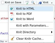
Comment générer un rapport à partager avec R ?

R permet d’automatiser des calculs, mais aussi de générer des rapports sous différents formats qui peuvent être facilement partagés (HTML, PDF, etc). Cela se fait grâce à R Markdown (intégré dans RStudio)(cela correspond aux fichiers .Rmd).

R Markdown permet d’écrire son script R pour réaliser les actions souhaitées et d’afficher dans le même document le résultat des actions. Ainsi, il est possible d’afficher uniquement le résultat final souhaité, composé de textes, de tableaux, de graphiques, etc.

Le code Rmarkdown permettant de générer un rapport avec des visualisations de données commence par aller chercher les données qui sont dans un fichier à sélectionner (il s’agit d’un fichier contenant les réponses à un sondage de satisfaction avec les colonnes Date, Motif de visite, Note de satisfaction).

Un document Rmarkdown commence par un bloc contenant les infos du titre du document et d’eventuels parametres à prendre en compte ou à proposer à l’utilisateur (ce bloc commence et finit par ‘- – -‘).

Pour créer des parties dans le documents, il est possible de définir des titres de parties avec « ## » (par exemple : ## Mon Titre de Partie).

Les blocs executant du code R commencent et finissent par 3 backquotes (« `). Il est possible de définir dans les paramètres du bloc (via les {}) si on souhaite que le code R soit affiché ou non dans le document final qui sera généré. Pour ne pas afficher le code, on met include=FALSE. Ainsi, seul le résultat final (correspondant à ce qui serait affiché dans la console) est affiché dans le document généré. A noter que dans ces blocs où le code R est éxécuté, le caractère # correspond à des commentaires.

Pour générer des graphiques, il s’agit de faire appel à la librairie ggplot2. Pour afficher des tableaux de données, il s’agit de passer par la fonction kable de la librairie knitr (knitr::kable()).

Le code du document .Rmd génère le document HTML suivant :

Visualisation-des-reponses-au-sondage Télécharger

Ci-dessous le code Rmarkdown permettant de générer le rapport :

1---
2title: "Visualisation des reponses au sondage"
3output: html_document
4params:
5  CompleteAnswersOnly:
6    label: "Ne prendre en compte que les réponses complètes:"
7    value: NON
8    input: select
9    choices: [NON,OUI]
10 
11---
12 
13 
14```{r setup, include=FALSE}
15knitr::opts_chunk$set(echo = FALSE)
16```
17 
18 
19```{r echo = FALSE, warning = FALSE, message = FALSE}
20 
21#Librairies necessaires 
22###########################
23 
24library(dplyr) 
25library(stringr)
26library(ggplot2)
27library(glue)
28library(tidyselect)
29library(scales)
30library(plotly)
31 
32#Preparation des donnees 
33###########################
34 
35# Chemin d acces au fichier
36chemin_fichier <- choose.files(caption="Selectionner le fichier de donnees")
37chemin_fichier <- chemin_fichier[1]
38 
39# Import des données à partir du fichier txt (tab)
40data_sondage <- read.delim(chemin_fichier, sep ="\t")
41 
42# FONCTION pour formatter le texte
43formatter_texte <- function(texte){
44  texte <- texte %>% str_replace_all("[.]", "_") %>% str_replace_all(' ','_') %>% str_replace_all("'","_")  %>% str_replace_all("-","_") %>% str_replace_all("/","_") %>% str_replace_all(",","_") %>% str_replace_all("[(]","_") %>% str_replace_all("[)]","_") %>% enc2native() %>% iconv(to='ASCII//TRANSLIT')
45  return(texte)
46}
47 
48# Renommer les champs (remplacer les points par des underscores)
49colnames(data_sondage) <- formatter_texte(colnames(data_sondage))
50 
51# Pour le parametre CompleteAnswerOnly
52if(params$CompleteAnswersOnly == "OUI"){
53  data_visualisation <- data_sondage %>% filter(Statut == "Complet" )
54} else {
55  data_visualisation <- data_sondage
56}
57 
58#Affichage du tableau de données
59glue("Les réponses au sondage :")
60knitr::kable(data_visualisation, align=rep('c', 3))
61 
62```
63 
64 
65## Infos sur le sondage
66 
67```{r echo = FALSE, warning = FALSE, message = FALSE}
68 
69#Generation du texte et des graphiques 
70###########################
71 
72# Periode du questionnaire
73dtMin <- data_visualisation[["Date"]] %>% as.Date(format = "%d/%m/%Y") %>% min() %>% format(format="%d/%m/%Y")
74dtMax <- data_visualisation[["Date"]] %>% as.Date(format = "%d/%m/%Y") %>% max() %>% format(format="%d/%m/%Y")
75glue("Periode de collecte des reponses : Du {dtMin} au {dtMax}")
76 
77# Rappel des parametres
78glue("Rappel des parametres : 
79     - Prendre en compte que les réponses complètes : {params$CompleteAnswersOnly}
80     ")
81 
82```
83 
84 
85## Satisfaction
86 
87```{r echo = FALSE, warning = FALSE, message = FALSE}
88 
89# Nombre reponses a la question de satisfaction
90nom_question <- "Quelle_est_votre_satisfaction"
91nb_rep <- data_visualisation[nom_question] %>% filter(is.na(.data[[nom_question]]) == FALSE & .data[[nom_question]] != "") %>% nrow()
92glue("Nombre de repondants à la question : {nb_rep}")
93 
94 
95# FONCTION pour generer les graphiques simples
96visualisation_barres <- function(data_visualisation, nom_question, color_fill = "#AED6F1", tri_asc = TRUE, tri_aide = FALSE){
97  # Formatter le nom de question pour qu il corresponde a celui de la table
98  nom_question <- formatter_texte(nom_question)
99  # Préparation du tableau pour decompte
100  # Recuperation des reponses possible (en valeur brute, differente de la valeur dans le nom de colonne)
101  index_colonne_question <- which(colnames(data_visualisation) == nom_question)
102  reponses_possibles <- data_visualisation[nom_question] %>% unique()
103  # Compiler les decomptes dans une table pour les visualisation
104  data_graph <- data_visualisation[] %>% filter(.data[[nom_question]] != "") %>% count(.data[[nom_question]])
105  colnames(data_graph)[1] <- "Reponse"
106  colnames(data_graph)[2] <- "Decompte"
107  # Ajout du nombre de repondants pour calculer le ratio
108  total_repondants <- data_visualisation[ data_visualisation[nom_question] != "" ,index_colonne_question] %>% length()
109  data_graph[,3] <- total_repondants %>% as.numeric()
110  colnames(data_graph)[3] <- 'Total_repondants'
111  data_graph[,4] <- data_graph[,2] / data_graph[,3]
112  colnames(data_graph)[4] <- 'Ratio'
113  ## Tri de donnees du plus petit au plus grand
114  if( tri_asc == TRUE){
115    aide_data_graph <- data_graph %>% arrange(desc(Ratio)) %>% select(Reponse)
116    data_graph <- data_graph %>% mutate(Reponse=factor(Reponse, levels=aide_data_graph[["Reponse"]]))
117  } else if(tri_asc == "CUSTOM" & is.vector(tri_aide) == TRUE){
118    data_graph <- data_graph %>% mutate(Reponse=factor(Reponse, levels=tri_aide))
119  }
120  #
121  # Generation du graphique
122  #
123  graph_question <- ggplot(data=data_graph, aes(x=Reponse, y=Ratio)) +
124     geom_bar(stat="identity", width = 0.5, fill = color_fill) +
125     # ggtitle(titre) +
126     theme_minimal() +
127     coord_flip() +
128     theme(axis.text.x = element_text(angle = 0, hjust = 1, vjust=1)) +
129     theme( axis.title.x = element_blank(), axis.title.y = element_blank() ) +
130     scale_y_continuous(labels=scales::percent) 
131  # Retourner le graphique a la fin
132  return(graph_question )
133}
134 
135 
136#
137# 1ere partie
138#
139 
140nom_question <- "Quelle_est_votre_satisfaction"
141visualisation_barres(data_visualisation, nom_question, tri_asc=FALSE, color_fill="#A6ACAF") %>% ggplotly() %>% config(modeBarButtonsToRemove = c("lasso2d", "pan2d", "zoom2d"))
142 
143#
144# 2eme partie
145#
146 
147# FONCTION pour barres avec 2eme champ
148visualisation_barres_avec_2eme_champ_filtre <- function(data_visualisation, nom_question, deuxieme_champ, color_fill = "#AED6F1", tri_asc = TRUE, tri_aide = FALSE){
149  # Formatter le nom de question pour qu il corresponde a celui de la table
150  nom_question <- formatter_texte(nom_question)
151  # Préparation du tableau pour decompte
152  # Recuperation des reponses possible (en valeur brute, differente de la valeur dans le nom de colonne)
153  index_colonne_question <- which(colnames(data_visualisation) == nom_question)
154  index_deuxieme_champ <- which(colnames(data_visualisation) == deuxieme_champ)
155  reponses_possibles <- data_visualisation[nom_question] %>% unique()
156  # Compiler les decomptes dans une table pour les visualisation
157  data_graph <- data_visualisation[] %>% filter(.data[[nom_question]] != "" & .data[[deuxieme_champ]] != "") %>% count(.data[[nom_question]])
158  colnames(data_graph)[1] <- "Reponse"
159  colnames(data_graph)[2] <- "Decompte"
160  # Ajout du nombre de repondants pour calculer le ratio
161  total_repondants <- data_visualisation[ data_visualisation[deuxieme_champ] != "" ,index_deuxieme_champ] %>% length()
162  data_graph[,3] <- total_repondants %>% as.numeric()
163  colnames(data_graph)[3] <- 'Total_repondants'
164  data_graph[,4] <- data_graph[,2] / data_graph[,3]
165  colnames(data_graph)[4] <- 'Ratio'
166  # Tri de donnees du plus petit au plus grand
167  if( tri_asc == TRUE){
168    aide_data_graph <- data_graph %>% arrange(Ratio) %>% select(Reponse) %>% unique()
169    data_graph <- data_graph %>% mutate(Reponse=factor(Reponse, levels=aide_data_graph[["Reponse"]]))
170  } else if(tri_asc == "CUSTOM" & is.vector(tri_aide) == TRUE){
171    data_graph <- data_graph %>% mutate(Reponse=factor(Reponse, levels=tri_aide))
172  }
173  #
174  # Generation du graphique
175  #
176  graph_question <- ggplot(data=data_graph, aes(x=Reponse, y=Ratio)) +
177    geom_bar(stat="identity", width = 0.5, fill = color_fill) +
178    # ggtitle(titre) +
179    theme_minimal() +
180    coord_flip() +
181    theme(axis.text.x = element_text(angle = 0, hjust = 1, vjust=1)) +
182    theme( axis.title.x = element_blank(), axis.title.y = element_blank() ) +
183    scale_y_continuous(labels=percent) 
184  # Retourner le graphiquea la fin
185  return(graph_question )
186}
187 
188# Graph1 - Pour le motif
189nom_question <- "Quel_est_votre_motif_de_visite"
190deuxieme_champ <- "Quelle_est_votre_satisfaction"
191graph1 <- visualisation_barres_avec_2eme_champ_filtre(data_visualisation, nom_question, deuxieme_champ) %>% ggplotly() %>% config(modeBarButtonsToRemove = c("lasso2d", "pan2d", "zoom2d"))
192 
193# FONCTION pour barres empilees
194visualisation_barres_empiles <- function(data_visualisation, nom_question, champ_remplissage, libelle_axe = TRUE, color_fill = c("#28B463", "#A9DFBF","#F9EBEA", "#F1948A","#CB4335")){
195  # Formatter le nom de question pour qu il corresponde a celui de la table
196  nom_question <- formatter_texte(nom_question)
197  # Préparation du tableau pour visualisation avec 1 data frame par question et transposition du decompte des valeurs en ligne
198  # Recuperation des colonnes a utiliser
199  index_colonne_question <- which(colnames(data_visualisation) == nom_question)
200  index_champ_remplissage <- which(colnames(data_visualisation) == champ_remplissage)
201  data_graph <- data_visualisation[] %>% filter(.data[[nom_question]] != "" & .data[[champ_remplissage]] != "") %>% count(.data[[nom_question]], .data[[champ_remplissage]])
202  colnames(data_graph)[1] <- "Reponse"
203  colnames(data_graph)[2] <- "Note"
204  colnames(data_graph)[3] <- "Decompte"
205  # Ajout du nombre de repondants pour calculer le ratio
206  total_repondants <- data_visualisation[ data_visualisation[champ_remplissage] != "" ,index_champ_remplissage] %>% length()
207  data_graph[,4] <- total_repondants %>% as.numeric()
208  colnames(data_graph)[4] <- 'Total_repondants'
209  data_graph[,5] <- data_graph[,3] / data_graph[,4]
210  colnames(data_graph)[5] <- 'Ratio'
211  # Ordre de donnees du plus petit au plus grand
212  aide_data_reponse <- data_graph %>% group_by(Reponse) %>% summarise(Ratio=sum(Ratio)) %>% arrange(Ratio) %>% select(Reponse)
213  data_graph <- data_graph %>% mutate(Reponses=factor(Reponse, levels=aide_data_reponse[["Reponse"]]))
214  # Ordre des libellés de satisfaction (color_fill)
215  aide_data_note <- data_graph %>% select(Note) %>% unique() %>% arrange(desc(Note))
216  data_graph <- data_graph %>% mutate(Notes=factor(Note, levels=aide_data_note[["Note"]]))
217  #
218  # Generation du graphique
219  #
220  if(libelle_axe == TRUE){
221    graph_question <- ggplot(data=data_graph, aes(x=Reponses, y=Decompte, fill=Notes)) +
222      geom_bar(position="fill", stat="identity") +
223      theme_minimal() +
224      coord_flip() +
225      theme(axis.text.y = element_text(angle = 0, hjust = 1, vjust=1), legend.position = "top", legend.title=element_blank(), axis.title.x = element_blank(), axis.title.y = element_blank()) +
226      scale_y_continuous(labels=percent) +
227      scale_fill_manual(values=color_fill)
228  } else {
229    graph_question <- ggplot(data=data_graph, aes(x=Reponses, y=Decompte, fill=Notes)) +
230      geom_bar(position="fill", stat="identity") +
231      theme_minimal() +
232      coord_flip() +
233      theme(axis.text.y = element_blank(), legend.position = "top", legend.title=element_blank(), axis.title.x = element_blank(), axis.title.y = element_blank()) +
234      scale_y_continuous(labels=percent) +
235      scale_fill_manual(values=color_fill)
236  }
237  # Retourner le graphique a la fin
238  return(graph_question)
239}
240 
241# FONCTION pour gerer la legende avec plotly
242reverse_legend_labels <- function(plotly_plot) {
243  n_labels <- length(plotly_plot$x$data)
244  plotly_plot$x$data[1:n_labels] <- plotly_plot$x$data[n_labels:1]
245  plotly_plot
246}
247 
248# Graph2 - Pour le motif détaillé par la satisfaction
249nom_question <- "Quel_est_votre_motif_de_visite"
250champ_remplissage <- "Quelle_est_votre_satisfaction"
251graph2 <- visualisation_barres_empiles(data_visualisation, nom_question, champ_remplissage, libelle_axe=FALSE) %>% ggplotly() %>% reverse_legend_labels() %>% layout(legend = list(orientation = "h", x = 0, y = 1.2)) %>% config(modeBarButtonsToRemove = c("lasso2d", "pan2d", "zoom2d"))
252 
253# Affichage dans une grille pour que les graphiques soient cote a cote
254subplot(graph1, graph2, widths = c(0.2, 0.8))  %>% layout(autosize = FALSE, width = 900)
255 
256#
257# 3eme partie
258#
259 
260# Tableau de la note moyenne par motif
261glue("Note moyenne par motif de visite :")
262# Transformation des reponses de satisfaction de texte en numerique
263notes <- data_visualisation[["Quelle_est_votre_satisfaction"]] %>% str_sub(1,1) %>% as.numeric()
264# Calcul des notes moyenne et tri desc
265data_tableau <- data_visualisation %>% mutate(notes=notes) %>% filter(is.na(notes) == FALSE) %>% group_by(Quel_est_votre_motif_de_visite) %>% summarise(note_moyenne = mean(notes)) %>% arrange(desc(note_moyenne))
266# Affichage du tableau avec les donnees
267knitr::kable(data_tableau, align=rep('c', 3))
268 
269 
270```
271 
272 
273***
274 
275## FIN du rapport

Et pour générer ce document HTML de manière dynamique avec du code R, il s’agit de faire appel à ce code qui génère un fichier .md à partir du fichier .Rmd (via knit), puis le fichier HTML est généré à partir du fichier .md :

1require(knitr)
2require(markdown)
3require(rmarkdown)
4knit('monfichier.Rmd', 'monfichier.md')
5markdownToHTML('monfichier.md', 'monfichier.html')

Pour + d’infos :

https://rmarkdown.rstudio.com/lesson-1.html

https://rstudio.github.io/cheatsheets/rmarkdown.pdf

0.00 avg. rating (0% score) - 0 votes

Laissez un commentaire Annuler la réponse